Grim SlashOverview:
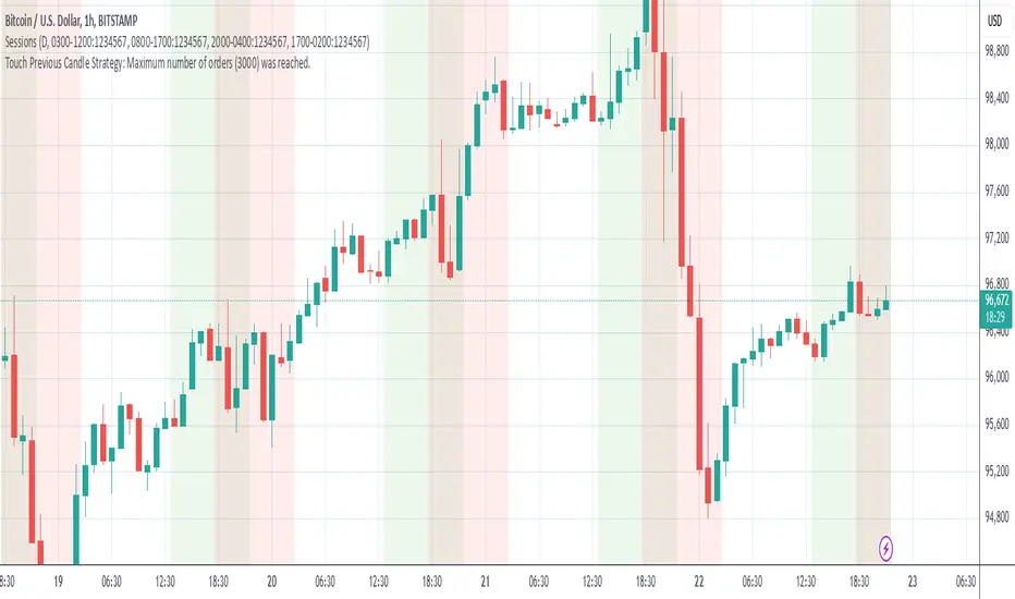
The Touch Previous Candle Strategy is a simple yet effective trading approach designed for the 1-hour chart. It focuses on price action by placing trades when the current candle interacts with key levels from the previous candle. The strategy is fully automated and includes risk management with take profit and stop loss levels.
Entry Conditions:
Buy Signal: A buy order is triggered when the low of the current candle touches or drops below the previous candle's closing price.
Sell Signal: A position is closed when the high of the current candle reaches or exceeds the previous candle's highest price.
Risk Management:
Take Profit: The trade is exited automatically when the price increases by 15% from the entry point.
Stop Loss: A stop loss is set at 5% below the entry price to minimize risk.
Best Use Cases:
Works well in volatile markets where price frequently tests previous levels.
Suitable for traders who prefer price-action-based strategies over indicators.
Can be optimized for different assets or timeframes based on market behavior.
Cari dalam skrip untuk "the strat"
Cash And Carry Arbitrage BTC Compare Month 6 by SeoNo1Detailed Explanation of the BTC Cash and Carry Arbitrage Script
Script Title: BTC Cash And Carry Arbitrage Month 6 by SeoNo1
Short Title: BTC C&C ABT Month 6
Version: Pine Script v5
Overlay: True (The indicators are plotted directly on the price chart)
Purpose of the Script
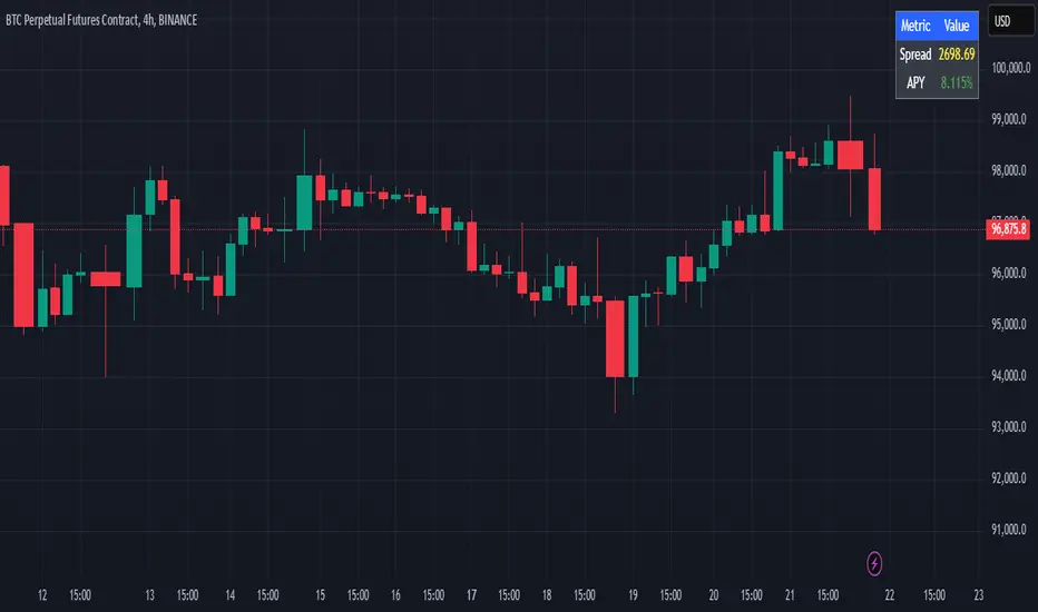
This script is designed to help traders analyze and track arbitrage opportunities between the spot market and futures market for Bitcoin (BTC). Specifically, it calculates the spread and Annual Percentage Yield (APY) from a cash-and-carry arbitrage strategy until a specific expiry date (in this case, June 27, 2025).
The strategy helps identify profitable opportunities when the futures price of BTC is higher than the spot price. Traders can then buy BTC in the spot market and short BTC futures contracts to lock in a risk-free profit.
1. Input Settings
Spot Symbol: The real-time BTC spot price from Binance (BTCUSDT).
Futures Symbol: The BTC futures contract that expires in June 2025 (BTCUSDM2025).
Expiry Date: The expiration date of the futures contract, set to June 27, 2025.
These inputs allow users to adjust the symbols or expiry date according to their trading needs.
2. Price Data Retrieval
Spot Price: Fetches the latest closing price of BTC from the spot market.
Futures Price: Fetches the latest closing price of BTC futures.
Spread: The difference between the futures price and the spot price (futures_price - spot_price).
The spread indicates how much higher (or lower) the futures price is compared to the spot market.
3. Time to Maturity (TTM) and Annual Percentage Yield (APY) Calculation
Current Date: Gets the current timestamp.
Time to Maturity (TTM): The number of days left until the futures contract expires.
APY Calculation:
Formula:
APY = ( Spread / Spot Price ) x ( 365 / TTM Days ) x 100
This represents the annualized return from holding a cash-and-carry arbitrage position if the trader buys BTC at the spot price and sells BTC futures.
4. Display Information Table on the Chart
A table is created on the chart's top-right corner showing the following data:
Metric: Labels such as Spread and APY
Value: Displays the calculated spread and APY
The table automatically updates at the latest bar to display the most recent data.
5. Alert Condition
This sets an alert condition that triggers every time the script runs.
In practice, users can modify this alert to trigger based on specific conditions (e.g., APY exceeds a threshold).
6. Plotting the APY and Spread
APY Plot: Displays the annualized yield as a blue line on the chart.
Spread Plot: Visualizes the futures-spot spread as a red line.
This helps traders quickly identify arbitrage opportunities when the spread or APY reaches desirable levels.
How to Use the Script
Monitor Arbitrage Opportunities:
A positive spread indicates a potential cash-and-carry arbitrage opportunity.
The larger the APY, the more profitable the arbitrage opportunity could be.
Timing Trades:
Execute a buy on the BTC spot market and simultaneously sell BTC futures when the APY is attractive.
Close both positions upon futures contract expiry to realize profits.
Risk Management:
Ensure you have sufficient margin to hold both positions until expiry.
Monitor funding rates and volatility, which could affect returns.
Conclusion
This script is an essential tool for traders looking to exploit price discrepancies between the BTC spot market and futures market through a cash-and-carry arbitrage strategy. It provides real-time data on spreads, annualized returns (APY), and visual alerts, helping traders make informed decisions and maximize their profit potential.
Boilerplate Configurable Strategy [Yosiet]This is a Boilerplate Code!
Hello! First of all, let me introduce myself a little bit. I don't come from the world of finance, but from the world of information and communication technologies (ICT) where we specialize in data processing with the aim of automating it and eliminating all human factors and actors in the processes. You could say that I am an algotrader.
That said, in my journey through trading in recent years I have understood that this world is often shown to be incomplete. All those who want to learn about trading only end up learning a small part of what it really entails, they only seek to learn how to read candlesticks. Therefore, I want to share with the entire community a fraction of what I have really understood it to be.
As a computer scientist, the most important thing is the data, it is the raw material of our work and without data you simply cannot do anything. Entropy is simple: Data in -> Data is transformed -> Data out.
The quality of the outgoing data will directly depend on the incoming data, there is no greater mystery or magic in the process. In trading it is no different, because at the end of the day it is nothing more than data. As we often say, if garbage comes in, garbage comes out.
Most people focus on the results only, on the outgoing data, because in the end we all want the same thing, to make easy money. Very few pay attention to the input data, much less to the process.
Now, I am not here to delude you, because there is no bigger lie than easy money, but I am here to give you a boilerplate code that will help you create strategies where you only have to concentrate on the quality of the incoming data.
To the Point
The code is a strategy boilerplate that applies the technique that you decide to customize for the criteria for opening a position. It already has the other factors involved in trading programmed and automated.
1. The Entry
This section of the boilerplate is the one that each individual must customize according to their needs and knowledge. The code is offered with two simple, well-known strategies to exemplify how the code can be reused for your own benefits.
For the purposes of this post on tradingview, I am going to use the simplest of the known strategies in trading for entries: SMA Crossing
// SMA Cross Settings
maFast = ta.sma(close, length)
maSlow = ta.sma(open, length)
The Strategy Properties for all cases published here:
For Stock TSLA H1 From 01/01/2025 To 02/15/2025
For Crypto XMR-USDT 30m From 01/01/2025 To 02/15/2025
For Forex EUR-USD 5m From 01/01/2025 To 02/15/2025
But the goal of this post is not to sell you a dream, else to show you that the same Entry decision works very well for some and does not for others and with this boilerplate code you only have to think of entries, not exits.
2. Schedules, Days, Sessions
As you know, there are an infinite number of markets that are susceptible to the sessions of each country and the news that they announce during those sessions, so the code already offers parameters so that you can condition the days and hours of operation, filter the best time parameters for a specific market and time frame.
3. Data Filtering
The data offered in trading are numerical series presented in vectors on a time axis where an endless number of mathematical equations can be applied to process them, with matrix calculation and non-linear regressions being the best, in my humble opinion.
4. Read Fundamental Macroeconomic Events, News
The boilerplate has integration with the tradingview SDK to detect when news will occur and offers parameters so that you can enable an exclusion time margin to not operate anything during that time window.
5. Direction and Sense
In my experience I have found the peculiarity that the same algorithm works very well for a market in a time frame, but for the same market in another time frame it is only a waste of time and money. So now you can easily decide if you only want to open LONG, SHORT or both side positions and know how effective your strategy really is.
6. Reading the money, THE PURPOSE OF EVERYTHING
The most important section in trading and the reason why many clients usually hire me as a financial programmer, is reading and controlling the money, because in the end everyone wants to win and no one wants to lose. Now they can easily parameterize how the money should flow and this is the genius of this boilerplate, because it is what will really decide if an algorithm (Indicator: A bunch of math equations) for entries will really leave you good money over time.
7. Managing the Risk, The Ego Destroyer
Many trades, little money. Most traders focus on making money and none of them know about statistics and the few who do know something about it, only focus on the winrate. Well, with this code you can unlock what really matters, the true success criteria to be able to live off of trading: Profit Factor, Sortino Ratio, Sharpe Ratio and most importantly, will you really make money?
8. Managing Emotions
Finally, the main reason why many lose money is because they are very bad at managing their emotions, because with this they will no longer need to do so because the boilerplate has already programmed criteria to chase the price in a position, cut losses and maximize profits.
In short, this is a boilerplate code that already has the data processing and data output ready, you only have to worry about the data input.
“And so the trader learned: the greatest edge was not in predicting the storm, but in building a boat that could not sink.”
DISCLAIMER
This post is intended for programmers and quantitative traders who already have a certain level of knowledge and experience. It is not intended to be financial advice or to sell you any money-making script, if you use it, you do so at your own risk.

CBC Strategy with Trend Confirmation & Separate Stop LossCBC Flip Strategy with Trend Confirmation and ATR-Based Targets
This strategy is based on the CBC Flip concept taught by MapleStax and inspired by the original CBC Flip indicator by AsiaRoo. It focuses on identifying potential reversals or trend continuation points using a combination of candlestick patterns (CBC Flips), trend filters, and a time-based entry window. This approach helps traders avoid false signals and increase trade accuracy.
What is a CBC Flip?
The CBC Flip is a candlestick-based pattern that identifies moments when the market is likely to change direction or strengthen its trend. It checks for a shift in price behavior between consecutive candles, signaling a bullish (upward) or bearish (downward) move.
However, not all flips are created equal! This strategy differentiates between Strong Flips and All Flips, allowing traders to choose between a more conservative or aggressive approach.
Strong Flips vs. All Flips
Strong Flips
A Strong Flip is a high-probability setup that occurs only after liquidity is swept from the previous candle’s high or low.
What is a liquidity sweep? This happens when the price briefly moves beyond the high or low of the previous candle, triggering stop-losses and trapping traders in the wrong direction. These sweeps often create fuel for the next move, making them powerful reversal signals.
Examples:
Long Setup: The price dips below the previous candle’s low (sweeping liquidity) and then closes higher, signaling a potential bullish move.
Short Setup: The price moves above the previous candle’s high and then closes lower, signaling a potential bearish move.
Why Use Strong Flips?
They provide fewer signals, but the accuracy is generally higher.
Ideal for trending markets where liquidity sweeps often mark key turning points.
All Flips
All Flips are less selective, offering both Strong Flips and additional signals without requiring a liquidity sweep.
This approach gives traders more frequent opportunities but comes with a higher risk of false signals, especially in sideways markets.
Examples:
Long Setup: A CBC flip occurs without sweeping the previous low, but the trend direction is confirmed (slow EMA is still above VWAP).
Short Setup: A CBC flip occurs without sweeping the previous high, but the trend is still bearish (slow EMA below VWAP).
Why Use All Flips?
Provides more frequent entries for active or aggressive traders.
Works well in trending markets but requires caution during consolidation periods.
How This Strategy Works
The strategy combines CBC Flips with multiple filters to ensure better trade quality:
Trend Confirmation: The slow EMA (20-period) must be positioned relative to the VWAP to confirm the overall trend direction.
Long Trades: Slow EMA must be above VWAP (upward trend).
Short Trades: Slow EMA must be below VWAP (downward trend).
Time-Based Filter: Traders can specify trading hours to limit entries to a particular time window, helping avoid low-volume or high-volatility periods.
Profit Target and Stop-Loss:
Profit Target: Defined as a multiple of the 14-period ATR (Average True Range). For example, if the ATR is 10 points and the profit target multiplier is set to 1.5, the strategy aims for a 15-point profit.
Stop-Loss: Uses a dynamic, candle-based stop-loss:
Long Trades: The trade closes if the market closes below the low of two candles ago.
Short Trades: The trade closes if the market closes above the high of two candles ago.
This approach adapts to recent price behavior and protects against unexpected reversals.
Customizable Settings
Strong Flips vs. All Flips: Choose between a more selective or aggressive entry style.
Profit Target Multiplier: Adjust the ATR multiplier to control the distance for profit targets.
Entry Time Range: Define specific trading hours for the strategy.
Indicators and Visuals
Fast EMA (10-Period) – Black Line
Slow EMA (20-Period) – Red Line
VWAP (Volume-Weighted Average Price) – Orange Line
Visual Labels:
▵ (Triangle Up) – Marks long entries (buy signals).
▿ (Triangle Down) – Marks short entries (sell signals).
Credits
CBC Flip Concept: Inspired by MapleStax, who teaches this concept.
Original Indicator: Developed by AsiaRoo, this strategy builds on the CBC Flip framework with additional features for improved trade management.
Risks and Disclaimer
This strategy is for educational purposes only and does not constitute financial advice.
Trading involves significant risk and may result in the loss of capital. Past performance does not guarantee future results. Use this strategy in a simulated environment before applying it to live trading.

highs&lowsone of my first strategy: highs&lows
This strategy takes the highest high and the lowest low of a specified timeframe and specified bar count.
It will then takes the average between these two extremes to create a center line.
This creates a range of high middle and low.
Then the strategy takes the current market movement
which is the direct average(no specified timeframe and specified bar count) of the current high and low.
Using this "current market movement" within the range of high middle and low it determins when to buy and then sell the asset.
*********note***************
-this strategy is (bullish)
-works good with most futures assets that have volatility/ decent movement
(might add more details if I forget any)
(work in progress)

Son Model ICT [TradingFinder] HTF DOL H1 + Sweep M15 + FVG M1🔵 Introduction
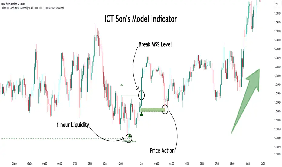
The ICT Son Model setup is a precise trading strategy based on market structure and liquidity, implemented across multiple timeframes. This setup first identifies a liquidity level in the 1-hour (1H) timeframe and then confirms a Market Structure Shift (MSS) in the 5-minute (5M) timeframe to validate the trend. After confirmation, the price forms a new swing in the 5-minute timeframe, absorbing liquidity.
Once this level is broken, traders typically drop to the 30-second (30s) timeframe and enter trades based on a Fair Value Gap (FVG). However, since access to the 30-second timeframe is not available to most traders, we take the entry signal directly from the 5-minute timeframe, using the same liquidity zones and confirmed breakouts to execute trades. This approach simplifies execution and makes the strategy accessible to all traders.
This model operates in two setups :
Bullish ICT Son Model and Bearish ICT Son Model. In the bullish setup, liquidity is first accumulated at the lows of the 1-hour timeframe, and after confirming a market structure shift, a long position is initiated. Conversely, in the bearish setup, liquidity is first drawn from higher levels, and upon confirmation of a bearish trend, a short position is executed.
Bullish Setup :
Bearish Setup :
🔵 How to Use
The ICT Son Model setup is designed around liquidity analysis and market structure shifts and can be applied in both bullish and bearish market conditions. The strategy first identifies a liquidity level in the 1-hour (1H) timeframe and then confirms a Market Structure Shift (MSS) in the 5-minute (5M) timeframe.
After this shift, the price forms a new swing, absorbing liquidity. When this level is broken in the 5-minute timeframe, the trader enters based on a Fair Value Gap (FVG). While the ideal entry is in the 30-second (30s) timeframe, due to accessibility constraints, we take entry signals directly from the 5-minute timeframe.
🟣 Bullish Setup
In the Bullish ICT Son Model, the 1-hour timeframe first identifies liquidity at the market lows, where price sweeps this level to absorb liquidity. Then, in the 5-minute timeframe, an MSS confirms the bullish shift.
After confirmation, the price forms a new swing, absorbing liquidity at a higher level. The price then retraces into a Fair Value Gap (FVG) created in the 5-minute timeframe, where the trader enters a long position, placing the stop-loss below the FVG.
🟣 Bearish Setup
In the Bearish ICT Son Model, liquidity at higher market levels is identified in the 1-hour timeframe, where price sweeps these levels to absorb liquidity. Then, in the 5-minute timeframe, an MSS confirms the bearish trend.
After confirmation, the price forms a new swing, absorbing liquidity at a lower level. The price then retraces into a Fair Value Gap (FVG) created in the 5-minute timeframe, where the trader enters a short position, placing the stop-loss above the FVG.
🔵 Settings
Swing period : You can set the swing detection period.
Max Swing Back Method : It is in two modes "All" and "Custom". If it is in "All" mode, it will check all swings, and if it is in "Custom" mode, it will check the swings to the extent you determine.
Max Swing Back : You can set the number of swings that will go back for checking.
FVG Length : Default is 120 Bar.
MSS Length : Default is 80 Bar.
FVG Filter : This refines the number of identified FVG areas based on a specified algorithm to focus on higher quality signals and reduce noise.
Types of FVG filters :
Very Aggressive Filter: Adds a condition where, for an upward FVG, the last candle's highest price must exceed the middle candle's highest price, and for a downward FVG, the last candle's lowest price must be lower than the middle candle's lowest price. This minimally filters out FVGs.
Aggressive Filter: Builds on the Very Aggressive mode by ensuring the middle candle is not too small, filtering out more FVGs.
Defensive Filter: Adds criteria regarding the size and structure of the middle candle, requiring it to have a substantial body and specific polarity conditions, filtering out a significant number of FVGs.
Very Defensive Filter: Further refines filtering by ensuring the first and third candles are not small-bodied doji candles, retaining only the highest quality signals.
🔵 Conclusion
The ICT Son Model setup is a structured and precise method for trade execution based on liquidity analysis and market structure shifts. This strategy first identifies a liquidity level in the 1-hour timeframe and then confirms a trend shift using the 5-minute timeframe.
Trade entries are executed based on Fair Value Gaps (FVGs), which highlight optimal entry points. By applying this model, traders can leverage existing market liquidity to enter high-probability trades. The bullish setup activates when liquidity is swept from market lows and a market structure shift confirms an upward trend, whereas the bearish setup is used when liquidity is drawn from market highs, confirming a downtrend.
This approach enables traders to identify high-probability trade setups with greater precision compared to many other strategies. Additionally, since access to the 30-second timeframe is limited, the strategy remains fully functional in the 5-minute timeframe, making it more practical and accessible for a wider range of traders.
MTF Signal XpertMTF Signal Xpert – Detailed Description
Overview:
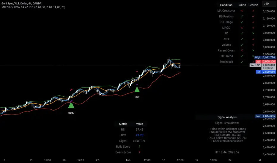
MTF Signal Xpert is a proprietary, open‑source trading signal indicator that fuses multiple technical analysis methods into one cohesive strategy. Developed after rigorous backtesting and extensive research, this advanced tool is designed to deliver clear BUY and SELL signals by analyzing trend, momentum, and volatility across various timeframes. Its integrated approach not only enhances signal reliability but also incorporates dynamic risk management, helping traders protect their capital while navigating complex market conditions.
Detailed Explanation of How It Works:
Trend Detection via Moving Averages
Dual Moving Averages:
MTF Signal Xpert computes two moving averages—a fast MA and a slow MA—with the flexibility to choose from Simple (SMA), Exponential (EMA), or Hull (HMA) methods. This dual-MA system helps identify the prevailing market trend by contrasting short-term momentum with longer-term trends.
Crossover Logic:
A BUY signal is initiated when the fast MA crosses above the slow MA, coupled with the condition that the current price is above the lower Bollinger Band. This suggests that the market may be emerging from a lower price region. Conversely, a SELL signal is generated when the fast MA crosses below the slow MA and the price is below the upper Bollinger Band, indicating potential bearish pressure.
Recent Crossover Confirmation:
To ensure that signals reflect current market dynamics, the script tracks the number of bars since the moving average crossover event. Only crossovers that occur within a user-defined “candle confirmation” period are considered, which helps filter out outdated signals and improves overall signal accuracy.
Volatility and Price Extremes with Bollinger Bands
Calculation of Bands:
Bollinger Bands are calculated using a 20‑period simple moving average as the central basis, with the upper and lower bands derived from a standard deviation multiplier. This creates dynamic boundaries that adjust according to recent market volatility.
Signal Reinforcement:
For BUY signals, the condition that the price is above the lower Bollinger Band suggests an undervalued market condition, while for SELL signals, the price falling below the upper Bollinger Band reinforces the bearish bias. This volatility context adds depth to the moving average crossover signals.
Momentum Confirmation Using Multiple Oscillators
RSI (Relative Strength Index):
The RSI is computed over 14 periods to determine if the market is in an overbought or oversold state. Only readings within an optimal range (defined by user inputs) validate the signal, ensuring that entries are made during balanced conditions.
MACD (Moving Average Convergence Divergence):
The MACD line is compared with its signal line to assess momentum. A bullish scenario is confirmed when the MACD line is above the signal line, while a bearish scenario is indicated when it is below, thus adding another layer of confirmation.
Awesome Oscillator (AO):
The AO measures the difference between short-term and long-term simple moving averages of the median price. Positive AO values support BUY signals, while negative values back SELL signals, offering additional momentum insight.
ADX (Average Directional Index):
The ADX quantifies trend strength. MTF Signal Xpert only considers signals when the ADX value exceeds a specified threshold, ensuring that trades are taken in strongly trending markets.
Optional Stochastic Oscillator:
An optional stochastic oscillator filter can be enabled to further refine signals. It checks for overbought conditions (supporting SELL signals) or oversold conditions (supporting BUY signals), thus reducing ambiguity.
Multi-Timeframe Verification
Higher Timeframe Filter:
To align short-term signals with broader market trends, the script calculates an EMA on a higher timeframe as specified by the user. This multi-timeframe approach helps ensure that signals on the primary chart are consistent with the overall trend, thereby reducing false signals.
Dynamic Risk Management with ATR
ATR-Based Calculations:
The Average True Range (ATR) is used to measure current market volatility. This value is multiplied by a user-defined factor to dynamically determine stop loss (SL) and take profit (TP) levels, adapting to changing market conditions.
Visual SL/TP Markers:
The calculated SL and TP levels are plotted on the chart as distinct colored dots, enabling traders to quickly identify recommended exit points.
Optional Trailing Stop:
An optional trailing stop feature is available, which adjusts the stop loss as the trade moves favorably, helping to lock in profits while protecting against sudden reversals.
Risk/Reward Ratio Calculation:
MTF Signal Xpert computes a risk/reward ratio based on the dynamic SL and TP levels. This quantitative measure allows traders to assess whether the potential reward justifies the risk associated with a trade.
Condition Weighting and Signal Scoring
Binary Condition Checks:
Each technical condition—ranging from moving average crossovers, Bollinger Band positioning, and RSI range to MACD, AO, ADX, and volume filters—is assigned a binary score (1 if met, 0 if not).
Cumulative Scoring:
These individual scores are summed to generate cumulative bullish and bearish scores, quantifying the overall strength of the signal and providing traders with an objective measure of its viability.
Detailed Signal Explanation:
A comprehensive explanation string is generated, outlining which conditions contributed to the current BUY or SELL signal. This explanation is displayed on an on‑chart dashboard, offering transparency and clarity into the signal generation process.
On-Chart Visualizations and Debug Information
Chart Elements:
The indicator plots all key components—moving averages, Bollinger Bands, SL and TP markers—directly on the chart, providing a clear visual framework for understanding market conditions.
Combined Dashboard:
A dedicated dashboard displays key metrics such as RSI, ADX, and the bullish/bearish scores, alongside a detailed explanation of the current signal. This consolidated view allows traders to quickly grasp the underlying logic.
Debug Table (Optional):
For advanced users, an optional debug table is available. This table breaks down each individual condition, indicating which criteria were met or not met, thus aiding in further analysis and strategy refinement.
Mashup Justification and Originality
MTF Signal Xpert is more than just an aggregation of existing indicators—it is an original synthesis designed to address real-world trading complexities. Here’s how its components work together:
Integrated Trend, Volatility, and Momentum Analysis:
By combining moving averages, Bollinger Bands, and multiple oscillators (RSI, MACD, AO, ADX, and an optional stochastic), the indicator captures diverse market dynamics. Each component reinforces the others, reducing noise and filtering out false signals.
Multi-Timeframe Analysis:
The inclusion of a higher timeframe filter aligns short-term signals with longer-term trends, enhancing overall reliability and reducing the potential for contradictory signals.
Adaptive Risk Management:
Dynamic stop loss and take profit levels, determined using ATR, ensure that the risk management strategy adapts to current market conditions. The optional trailing stop further refines this approach, protecting profits as the market evolves.
Quantitative Signal Scoring:
The condition weighting system provides an objective measure of signal strength, giving traders clear insight into how each technical component contributes to the final decision.
How to Use MTF Signal Xpert:
Input Customization:
Adjust the moving average type and period settings, ATR multipliers, and oscillator thresholds to align with your trading style and the specific market conditions.
Enable or disable the optional stochastic oscillator and trailing stop based on your preference.
Interpreting the Signals:
When a BUY or SELL signal appears, refer to the on‑chart dashboard, which displays key metrics (e.g., RSI, ADX, bullish/bearish scores) along with a detailed breakdown of the conditions that triggered the signal.
Review the SL and TP markers on the chart to understand the associated risk/reward setup.
Risk Management:
Use the dynamically calculated stop loss and take profit levels as guidelines for setting your exit points.
Evaluate the provided risk/reward ratio to ensure that the potential reward justifies the risk before entering a trade.
Debugging and Verification:
Advanced users can enable the debug table to see a condition-by-condition breakdown of the signal generation process, helping refine the strategy and deepen understanding of market dynamics.
Disclaimer:
MTF Signal Xpert is intended for educational and analytical purposes only. Although it is based on robust technical analysis methods and has undergone extensive backtesting, past performance is not indicative of future results. Traders should employ proper risk management and adjust the settings to suit their financial circumstances and risk tolerance.
MTF Signal Xpert represents a comprehensive, original approach to trading signal generation. By blending trend detection, volatility assessment, momentum analysis, multi-timeframe alignment, and adaptive risk management into one integrated system, it provides traders with actionable signals and the transparency needed to understand the logic behind them.
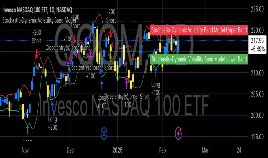
Stochastic-Dynamic Volatility Band ModelThe Stochastic-Dynamic Volatility Band Model is a quantitative trading approach that leverages statistical principles to model market volatility and generate buy and sell signals. The strategy is grounded in the concepts of volatility estimation and dynamic market regimes, where the core idea is to capture price fluctuations through stochastic models and trade around volatility bands.
Volatility Estimation and Band Construction
The volatility bands are constructed using a combination of historical price data and statistical measures, primarily the standard deviation (σ) of price returns, which quantifies the degree of variation in price movements over a specific period. This methodology is based on the classical works of Black-Scholes (1973), which laid the foundation for using volatility as a core component in financial models. Volatility is a crucial determinant of asset pricing and risk, and it plays a pivotal role in this strategy's design.
Entry and Exit Conditions
The entry conditions are based on the price’s relationship with the volatility bands. A long entry is triggered when the price crosses above the lower volatility band, indicating that the market may have been oversold or is experiencing a reversal to the upside. Conversely, a short entry is triggered when the price crosses below the upper volatility band, suggesting overbought conditions or a potential market downturn.
These entry signals are consistent with the mean reversion theory, which asserts that asset prices tend to revert to their long-term average after deviating from it. According to Poterba and Summers (1988), mean reversion occurs due to overreaction to news or temporary disturbances, leading to price corrections.
The exit condition is based on the number of bars that have elapsed since the entry signal. Specifically, positions are closed after a predefined number of bars, typically set to seven bars, reflecting a short-term trading horizon. This exit mechanism is in line with short-term momentum trading strategies discussed in literature, where traders capitalize on price movements within specific timeframes (Jegadeesh & Titman, 1993).
Market Adaptability
One of the key features of this strategy is its dynamic nature, as it adapts to the changing volatility environment. The volatility bands automatically adjust to market conditions, expanding in periods of high volatility and contracting when volatility decreases. This dynamic adjustment helps the strategy remain robust across different market regimes, as it is capable of identifying both trend-following and mean-reverting opportunities.
This dynamic adaptability is supported by the adaptive market hypothesis (Lo, 2004), which posits that market participants evolve their strategies in response to changing market conditions, akin to the adaptive nature of biological systems.
References:
Black, F., & Scholes, M. (1973). The Pricing of Options and Corporate Liabilities. Journal of Political Economy, 81(3), 637-654.
Bollinger, J. (1980). Bollinger on Bollinger Bands. Wiley.
Jegadeesh, N., & Titman, S. (1993). Returns to Buying Winners and Selling Losers: Implications for Stock Market Efficiency. Journal of Finance, 48(1), 65-91.
Lo, A. W. (2004). The Adaptive Markets Hypothesis: Market Efficiency from an Evolutionary Perspective. Journal of Portfolio Management, 30(5), 15-29.
Poterba, J. M., & Summers, L. H. (1988). Mean Reversion in Stock Prices: Evidence and Implications. Journal of Financial Economics, 22(1), 27-59.
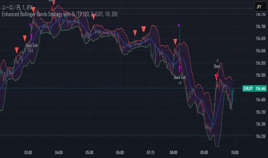
Enhanced Bollinger Bands Strategy with SL/TP// Title: Enhanced Bollinger Bands Strategy with SL/TP
// Description:
// This strategy is based on the classic Bollinger Bands indicator and incorporates Stop Loss (SL) and Take Profit (TP) levels for automated trading. It identifies potential long and short entry points based on price crossing the lower and upper Bollinger Bands, respectively. The strategy allows users to customize several parameters to suit different market conditions and risk tolerances.
// Key Features:
// * **Bollinger Bands:** Uses Simple Moving Average (SMA) as the basis and calculates upper and lower bands based on a user-defined standard deviation multiplier.
// * **Customizable Parameters:** Offers extensive customization, including SMA length, standard deviation multiplier, Stop Loss (SL) in pips, and Take Profit (TP) in pips.
// * **Long/Short Position Control:** Allows users to independently enable or disable long and short positions.
// * **Stop Loss and Take Profit:** Implements Stop Loss and Take Profit levels based on pip values to manage risk and secure profits. Entry prices are set to the band levels on signals.
// * **Visualizations:** Provides options to display Bollinger Bands and entry signals on the chart for easy analysis.
// Strategy Logic:
// 1. **Bollinger Bands Calculation:** The strategy calculates the Bollinger Bands using the specified SMA length and standard deviation multiplier.
// 2. **Entry Conditions:**
// * **Long Entry:** Enters a long position when the closing price crosses above the lower Bollinger Band and the `Enable Long Positions` setting is enabled.
// * **Short Entry:** Enters a short position when the closing price crosses below the upper Bollinger Band and the `Enable Short Positions` setting is enabled.
// 3. **Exit Conditions:**
// * **Stop Loss:** Exits the position if the price reaches the Stop Loss level, calculated based on the input `Stop Loss (Pips)`.
// * **Take Profit:** Exits the position if the price reaches the Take Profit level, calculated based on the input `Take Profit (Pips)`.
// Input Parameters:
// * **SMA Length (length):** The length of the Simple Moving Average used to calculate the Bollinger Bands (default: 20).
// * **Standard Deviation Multiplier (mult):** The multiplier applied to the standard deviation to determine the width of the Bollinger Bands (default: 2.0).
// * **Enable Long Positions (enableLong):** A boolean value to enable or disable long positions (default: true).
// * **Enable Short Positions (enableShort):** A boolean value to enable or disable short positions (default: true).
// * **Pip Value (pipValue):** The value of a pip for the traded instrument. This is crucial for accurate Stop Loss and Take Profit calculations (default: 0.0001 for most currency pairs). **Important: Adjust this value to match the specific instrument you are trading.**
// * **Stop Loss (Pips) (slPips):** The Stop Loss level in pips (default: 10).
// * **Take Profit (Pips) (tpPips):** The Take Profit level in pips (default: 20).
// * **Show Bollinger Bands (showBands):** A boolean value to show or hide the Bollinger Bands on the chart (default: true).
// * **Show Entry Signals (showSignals):** A boolean value to show or hide entry signals on the chart (default: true).
// How to Use:
// 1. Add the strategy to your TradingView chart.
// 2. Adjust the input parameters to optimize the strategy for your chosen instrument and timeframe. Pay close attention to the `Pip Value`.
// 3. Backtest the strategy over different periods to evaluate its performance.
// 4. Use the `Enable Long Positions` and `Enable Short Positions` settings to customize the strategy for specific market conditions (e.g., only long positions in an uptrend).
// Important Notes and Disclaimers:
// * **Backtesting Results:** Past performance is not indicative of future results. Backtesting results can be affected by various factors, including market volatility, slippage, and transaction costs.
// * **Risk Management:** This strategy is provided for informational and educational purposes only and should not be considered financial advice. Always use proper risk management techniques when trading. Adjust Stop Loss and Take Profit levels according to your risk tolerance.
// * **Slippage:** The strategy takes into account slippage by specifying a slippage parameter on the `strategy` declaration. However, real-world slippage may vary.
// * **Market Conditions:** The performance of this strategy can vary significantly depending on market conditions. It may perform well in trending markets but poorly in ranging or choppy markets.
// * **Pip Value Accuracy:** **Ensure the `Pip Value` is correctly set for the specific instrument you are trading. Incorrect pip value will result in incorrect stop loss and take profit placement.** This is critical.
// * **Broker Compatibility:** The strategy's performance may vary depending on your broker's execution policies and fees.
// * **Disclaimer:** I am not a financial advisor, and this script is not financial advice. Use this strategy at your own risk. I am not responsible for any losses incurred while using this strategy.
Moving Average Crossover StrategyCertainly! Below is an example of a professional trading strategy implemented in Pine Script for TradingView. This strategy is a simple moving average crossover strategy, which is a common approach used by many traders. It uses two moving averages (a short-term and a long-term) to generate buy and sell signals.
Input Parameters:
shortLength: The length of the short-term moving average.
longLength: The length of the long-term moving average.
Moving Averages:
shortMA: The short-term simple moving average (SMA).
longMA: The long-term simple moving average (SMA).
Conditions:
longCondition: A buy signal is generated when the short-term MA crosses above the long-term MA.
shortCondition: A sell signal is generated when the short-term MA crosses below the long-term MA.
Trade Execution:
The strategy enters a long position when the longCondition is met.
The strategy enters a short position when the shortCondition is met.
Plotting:
The moving averages are plotted on the chart.
Buy and sell signals are plotted as labels on the chart.
How to Use:
Copy the script into TradingView's Pine Script editor.
Adjust the shortLength and longLength parameters to fit your trading style.
Add the script to your chart and apply it to your desired timeframe.
Backtest the strategy to see how it performs on historical data.
This is a basic example, and professional traders often enhance such strategies with additional filters, risk management rules, and other indicators to improve performance.

Walk Forward PatternsINTRO
In Euclidean geometry, every mathematical output has a planar projection. 'Walk Forward Patterns' can be considered a practical example of this concept. On the other hand, this indicator might also be viewed as an experiment in 'how playing with Lego as a child contributes to time series analysis' :)
OVERVIEW
This script dynamically generates the necessary optimization and testing ranges for Walk Forward Analysis based on user-defined bar count and length inputs. It performs automatic calculations for each step, offers 8 different window options depending on the inputs, and visualizes the results dynamically. I should also note that most of the window models consist of original patterns I have created.
ADDITIONAL INFO : WHAT IS WALK FORWARD ANALYSIS?
Although it is not the main focus of this indicator, providing a brief definition of Walk Forward Analysis can be helpful in correctly interpreting the results it generates. Walk Forward Analysis (WFA) is a systematic method for optimizing parameters and validating trading strategies. It involves dividing historical data into variable segments, where a strategy is first optimized on an in-sample period and then tested on an out-of-sample period. This process repeats by shifting the windows forward, ensuring that each test evaluates the strategy on unseen data, helping to assess its robustness and adaptability in real market conditions.
ORIGINALITY
There are very few studies on Walk Forward Analysis in TradingView. Even worse, there are no any open-source studies available. Someone has to start somewhere, I suppose. And in my personal opinion, determining the optimization and backtest intervals is the most challenging part of WFA. These intervals serve as a prerequisite for automated parameter optimization. I felt the need to publish this pattern module, which I use in my own WFA models, partly due to this gap on community scripts.
INDICATOR MECHANICS
To use the indicator effectively, you only need to perform four simple tasks:
Specify the total number of bars in your chart in the 'Bar Index' parameter.
Define the optimization (In-Sample Test) length.
Define the testing (Out-Of-Sample Test) length.
Finally, select the window type.
The indicator automatically models everything else (including the number of steps) based on your inputs. And the result; you now have a clear idea of which bars to use for your Walk Forward tests!
A COMMONLY USED WINDOW SELECTION METHOD: ROLLING
A more concrete definition of Walk Forward Analysis, specifically for the widely used Rolling method, can be described as follows:
Parameters that have performed well over a certain period are identified (Optimization: In-Sample).
These parameters are then tested on a shorter, subsequent period (Backtest: Out-of-Sample).
The process is repeated forward in time (At each step, the optimization and backtest periods are shifted by the backtest length).
If the cumulative percentage profit obtained from the backtest results is greater than half of the historical optimization profit, the strategy is considered "successful."
If the strategy is successful, the most recent (untested) optimization values are used for live trading.
OTHER WINDOW OPTIONS
ANCHORED: That's a pattern based on progressively expanding optimization ranges at each step. Backtest ranges move forward in a staircase-like manner.
STATIC: Optimization ranges remain fixed, while backtest ranges are shifted forward.
BLOCKED: Optimization ranges are shifted forward in groups of three blocks. Backtest ranges are also shifted in a staircase manner, even at the cost of creating gaps from the optimization end bars.
TRIANGULAR: Optimization ranges are shifted forward in triangular regions, while backtest ranges move in a staircase pattern.
RATIO: The optimization length increases by 25% of the initial step’s fixed length at each step. In other words, the length grows by 25% of the first step's length incrementally. Backtest ranges always start from the bar where the optimization ends.
FIBONACCI: A variation of the Ratio method, where the optimization shift factor is set to 0.618
RANDOM WALK
Unlike the window models explained above, we can also generate optimization and backtest ranges completely randomly—offering almost unlimited variations! When you select the "Random" option in the "Window" parameter on the indicator interface, random intervals are generated based on various trigonometric calculations. By changing the numerical value in the '🐒' parameter, you can create entirely unique patterns.
WHY THE 🐒 EMOJI?
Two reasons.
First, I think that as humanity, we are a species of tailless primates who become happy when we understand things :). At least evolutionarily. The entire history of civilization is built on the effort to express the universe in a scale we can comprehend. 'Knowledge' is an invention born from this effort, which is why we feel happiness when we 'understand'. Second, I can't think of a better metaphor for randomness than a monkey sitting at a keyboard. See: Monkey Test.
Anyway, I’m rambling :)
NOTES
The indicator generates results for up to 100 steps. As the number of steps increases, the table may extend beyond the screen—don’t forget to zoom out!
FINAL WORDS
I haven’t published a Walk Forward script yet . However, there seem to be examples that can perform parameter optimization in the true sense of the word, producing more realistic results without falling into overfitting in my library. Hopefully, I’ll have the chance to publish one in the coming weeks. Sincerely thanks to Kıvanç Özbilgiç, Robert Pardo, Kevin Davey, Ernest P. Chan for their inspiring publishments.
DISCLAIMER
That's just a script, nothing more. I hope it helps everyone. Do not forget to manage your risk. And trade as safely as possible. Best of luck!
© dg_factor

The 950 Bar StrategyNQ 9:50 AM Candle Strategy v3 (Trade at 9:55AM) - 1 Contract
Also called the 950 Standard. The 950 Strategy.
This strategy places its trade at 9:55am each day based on the close of the 9:50am candle. Uses 5min timeframe candles. If candle closes red, or bearish, the strategy goes short. If candle closes green, or bullish, the strategy goes long. Brackets are 150tick TP and 200tick SL.

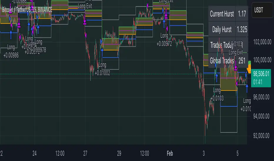
Advanced Multi-Timeframe Trading System (Risk Managed)Description:
This strategy is an original approach that combines two main analytical components to identify potential trade opportunities while simulating realistic trading conditions:
1. Market Trend Analysis via an Approximate Hurst Exponent
• What It Does:
The strategy computes a rough measure of market trending using an approximate Hurst exponent. A value above 0.5 suggests persistent, trending behavior, while a value below 0.5 indicates a tendency toward mean-reversion.
• How It’s Used:
The Hurst exponent is calculated on both the chart’s current timeframe and a higher timeframe (default: Daily) to capture both local and broader market dynamics.
2. Fibonacci Retracement Levels
• What It Does:
Using daily high and low data from a selected timeframe (default: Daily), the script computes key Fibonacci retracement levels.
• How It’s Used:
• The 61.8% level (Golden Ratio) serves as a key threshold:
• A long entry is signaled when the price crosses above this level if the daily Hurst exponent confirms a trending market.
• The 38.2% level is used to identify short-entry opportunities when the price crosses below it and the daily Hurst indicates non-trending conditions.
Signal Logic:
• Long Entry:
When the price crosses above the 61.8% Fibonacci level (Golden Ratio) and the daily Hurst exponent is greater than 0.5, suggesting a trending market.
• Short Entry:
When the price crosses below the 38.2% Fibonacci level and the daily Hurst exponent is less than 0.5, indicating a less trending or potentially reversing market.
Risk Management & Trade Execution:
• Stop-Loss:
Each trade is risk-managed with a stop-loss set at 2% below (for longs) or above (for shorts) the entry price. This ensures that no single trade risks more than a small, sustainable portion of the account.
• Take Profit:
A take profit order targets a risk-reward ratio of 1:2 (i.e., the target profit is twice the amount risked).
• Position Sizing:
Trades are executed with a fixed position size equal to 10% of account equity.
• Trade Frequency Limits:
• Daily Limit: A maximum of 5 trades per day
• Overall Limit: No more than 510 trades during the backtesting period (e.g., since 2019)
These limits are imposed to simulate realistic trading frequency and to avoid overtrading in backtest results.
Backtesting Parameters:
• Initial Capital: $10,000
• Commission: 0.1% per trade
• Slippage: 1 tick per bar
These settings aim to reflect the conditions faced by the average trader and help ensure that the backtesting results are realistic and not misleading.
Chart Overlays & Visual Aids:
• Fibonacci Levels:
The key Fibonacci retracement levels are plotted on the chart, and the zone between the 61.8% and 38.2% levels is highlighted to show a key retracement area.
• Market Trend Background:
The chart background is tinted green when the daily Hurst exponent indicates a trending market (value > 0.5) and red otherwise.
• Information Table:
An on-chart table displays key parameters such as the current Hurst exponent, daily Hurst value, the number of trades executed today, and the global trade count.
Disclaimer:
Past performance is not indicative of future results. This strategy is experimental and provided solely for educational purposes. It is essential that you backtest and paper trade using your own settings before considering any live deployment. The Hurst exponent calculation is an approximation and should be interpreted as a rough gauge of market behavior. Adjust the parameters and risk management settings according to your personal risk tolerance and market conditions.
Additional Notes:
• Originality & Usefulness:
This script is an original mashup that combines trend analysis with Fibonacci retracement methods. The description above explains how these components work together to provide trading signals.
• Realistic Results:
The strategy uses realistic account sizes, commission rates, slippage, and risk management rules to generate backtesting results that are representative of real-world trading.
• Educational Purpose:
This script is intended to support the TradingView community by offering insights into combining multiple analysis techniques in one strategy. It is not a “get-rich-quick” system but rather an educational tool to help traders understand risk management and trade signal logic.
By using this script, you acknowledge that trading involves risk and that you are responsible for testing and adjusting the strategy to fit your own trading environment. This publication is fully open source, and any modifications should include proper attribution if significant portions of the code are reused.
Arpeet MACDOverview
This strategy is based on the zero-lag version of the MACD (Moving Average Convergence Divergence) indicator, which captures short-term trends by quickly responding to price changes, enabling high-frequency trading. The strategy uses two moving averages with different periods (fast and slow lines) to construct the MACD indicator and introduces a zero-lag algorithm to eliminate the delay between the indicator and the price, improving the timeliness of signals. Additionally, the crossover of the signal line and the MACD line is used as buy and sell signals, and alerts are set up to help traders seize trading opportunities in a timely manner.
Strategy Principle
Calculate the EMA (Exponential Moving Average) or SMA (Simple Moving Average) of the fast line (default 12 periods) and slow line (default 26 periods).
Use the zero-lag algorithm to double-smooth the fast and slow lines, eliminating the delay between the indicator and the price.
The MACD line is formed by the difference between the zero-lag fast line and the zero-lag slow line.
The signal line is formed by the EMA (default 9 periods) or SMA of the MACD line.
The MACD histogram is formed by the difference between the MACD line and the signal line, with blue representing positive values and red representing negative values.
When the MACD line crosses the signal line from below and the crossover point is below the zero axis, a buy signal (blue dot) is generated.
When the MACD line crosses the signal line from above and the crossover point is above the zero axis, a sell signal (red dot) is generated.
The strategy automatically places orders based on the buy and sell signals and triggers corresponding alerts.
Advantage Analysis
The zero-lag algorithm effectively eliminates the delay between the indicator and the price, improving the timeliness and accuracy of signals.
The design of dual moving averages can better capture market trends and adapt to different market environments.
The MACD histogram intuitively reflects the comparison of bullish and bearish forces, assisting in trading decisions.
The automatic order placement and alert functions make it convenient for traders to seize trading opportunities in a timely manner, improving trading efficiency.
Risk Analysis
In volatile markets, frequent crossover signals may lead to overtrading and losses.
Improper parameter settings may cause signal distortion and affect strategy performance.
The strategy relies on historical data for calculations and has poor adaptability to sudden events and black swan events.
Optimization Direction
Introduce trend confirmation indicators, such as ADX, to filter out false signals in volatile markets.
Optimize parameters to find the best combination of fast and slow line periods and signal line periods, improving strategy stability.
Combine other technical indicators or fundamental factors to construct a multi-factor model, improving risk-adjusted returns of the strategy.
Introduce stop-loss and take-profit mechanisms to control single-trade risk.
Summary
The MACD Dual Crossover Zero Lag Trading Strategy achieves high-frequency trading by quickly responding to price changes and capturing short-term trends. The zero-lag algorithm and dual moving average design improve the timeliness and accuracy of signals. The strategy has certain advantages, such as intuitive signals and convenient operation, but also faces risks such as overtrading and parameter sensitivity. In the future, the strategy can be optimized by introducing trend confirmation indicators, parameter optimization, multi-factor models, etc., to improve the robustness and profitability of the strategy.
Swing Breakout System (SBS)The Swing Breakout Sequence (SBS) is a trading strategy that focuses on identifying high-probability entry points based on a specific pattern of price swings. This indicator will identify these patterns, then draw lines and labels to show confirmation.
How To Use:
The indicator will show both Bullish and Bearish SBS patterns.
Bullish Pattern is made up of 6 points: Low (0), HH (1), LL (2 | but higher than initial Low), New HH (3), LL (5), LL again (5)
Bearish Patten is made up of 6 points: High (0), LL (1), HH (2 | but lower than initial high), New LL (3), HH (5), HH again (5)
A label with an arrow will appear at the end, showing the completion of a successful sequence
Idea behind the strategy:
The idea behind this strategy, is the accumulation and then manipulation of liquidity throughout the sequence. For example, during SBS sequence, liquidity is accumulated during step (2), then price will push away to make a new high/low (step 3), after making a minor new high/low, price will retrace breaking the key level set up in step (2). This is price manipulating taking liquidity from behind high/low from step (2). After taking liquidity price the idea is price will continue in the original direction.
Step 0 - Setting up initial direction
Step 1 - Setting up initial direction
Step 2 - Key low/high establishing liquidity
Step 3 - Failed New high/low
Step 4 - Taking liquidity from step (2)
Step 5 - Taking liquidity from step 2 and 4
Pattern Detection:
- Uses pivot high/low points to identify swing patterns
- Stores 6 consecutive swing points in arrays
- Identifies two types of patterns:
1. Bullish Pattern: A specific sequence of higher lows and higher highs
2. Bearish Pattern: A specific sequence of lower highs and lower lows
Note: Because the indicator is identifying a perfect sequence of 6 steps, set ups may not appear frequently.
Visualization:
- Draws connecting lines between swing points
- Labels each point numerically (optional)
- Shows breakout arrows (↑ for bullish, ↓ for bearish)
- Generates alerts on valid breakouts
User Input Settings:
Core Parameters
1. Pivot Lookback Period (default: 2)
- Controls how many bars to look back/forward for pivot point detection
- Higher values create fewer but more significant pivot points
2. Minimum Pattern Height % (default: 0.1)
- Minimum required height of the pattern as a percentage of price
- Filters out insignificant patterns
3. Maximum Pattern Width (bars) (default: 50)
- Maximum allowed width of the pattern in bars
- Helps exclude patterns that form over too long a period

WAGMI LAB Trend Reversal Indicator HMA-Kahlman (m15)WAGMI HMA-Kahlman Trend Reversal Indicator
This indicator combines the Hull Moving Average (HMA) with the Kahlman filter to provide a dynamic trend reversal signal, perfect for volatile assets like Bitcoin. The strategy works particularly well on lower timeframes, making it ideal for intraday trading and fast-moving markets.
Key Features:
Trend Detection: It uses a blend of HMA and Kahlman filters to detect trend reversals, providing more accurate and timely signals.
Volatility Adaptability: Designed with volatile assets like Bitcoin in mind, this indicator adapts to rapid price movements, offering smoother trend detection during high volatility.
Easy Visualization: Buy (B) and Sell (S) signals are clearly marked with labels, helping traders spot trend shifts quickly and accurately.
Trendlines Module: The indicator plots trendlines based on pivot points, highlighting important support and resistance levels. This helps traders understand the market structure and identify potential breakout or breakdown zones.
Customizable: Adjust the HMA and Kahlman parameters to fit different assets or trading styles, making it flexible for various market conditions.
Usage Tips:
Best Timeframes: The indicator performs exceptionally well on lower timeframes (such as 15-minute to 1-hour charts), making it ideal for scalping and short-term trading strategies.
Ideal for Volatile Assets: This strategy is perfect for highly volatile assets like Bitcoin, but can also be applied to other cryptocurrencies and traditional markets with high price fluctuations.
Signal Confirmation: Use the trend signals (green for uptrend, red for downtrend) along with the buy/sell labels to help you confirm potential entries and exits. It's also recommended to combine the signals with other technical tools like volume analysis or RSI for enhanced confirmation.
Trendline Analysis: The plotted trendlines provide additional visual context to identify key market zones, supporting your trading decisions with a clear view of ongoing trends and possible reversal areas.
Risk Management: As with any strategy, always consider proper risk management techniques, such as stop-loss and take-profit levels, to protect against unforeseen market moves.

9-20 EMA Crossover with TP and SL9-20 EMA Crossover: This script tracks the crossover of the 9-period EMA and the 20-period EMA.
When the 9 EMA crosses above the 20 EMA, a buy signal is triggered.
When the 9 EMA crosses below the 20 EMA, a sell signal is triggered.
Take Profit and Stop Loss Levels:
The take profit for a long position is set at 3% above the entry price (close * 1.03).
The stop loss for a long position is set at 1% below the entry price (close * 0.99).
The take profit for a short position is set at 3% below the entry price (close * 0.97).
The stop loss for a short position is set at 1% above the entry price (close * 1.01).
Leverage: The strategy uses 20x leverage for both long and short positions (leverage=20).
Alerts: Alerts are set up for the buy signal when the 9 EMA crosses above the 20 EMA and the sell signal when the 9 EMA crosses below the 20 EMA. These alerts can be used with a webhook to trigger trades on Binance Futures.
Strategy:
For long trades: The strategy enters a long position and sets a take profit at 3% above the entry price and a stop loss at 1% below the entry price.
For short trades: The strategy enters a short position and sets a take profit at 3% below the entry price and a stop loss at 1% above the entry price.

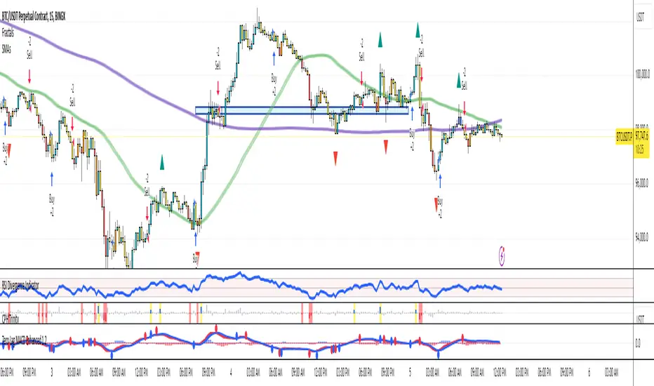
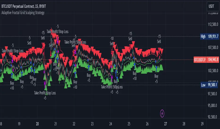
Adaptive Fractal Grid Scalping StrategyThis Pine Script v6 component implements an "Adaptive Fractal Grid Scalping Strategy" with an added volatility threshold feature.
Here's how it works:
Fractal Break Detection: Uses ta.pivothigh and ta.pivotlow to identify local highs and lows.
Volatility Clustering: Measures volatility using the Average True Range (ATR).
Adaptive Grid Levels: Dynamically adjusts grid levels based on ATR and user-defined multipliers.
Directional Bias Filter: Uses a Simple Moving Average (SMA) to determine trend direction.
Volatility Threshold: Introduces a new input to specify a minimum ATR value required to activate the strategy.
Trade Execution Logic: Places limit orders at grid levels based on trend direction and fractal levels, but only when ATR exceeds the volatility threshold.
Profit-Taking and Stop-Loss: Implements profit-taking at grid levels and a trailing stop-loss based on ATR.
How to Use
Inputs: Customize the ATR length, SMA length, grid multipliers, trailing stop multiplier, and volatility threshold through the input settings.
Visuals: The script plots fractal points and grid levels on the chart for easy visualization.
Trade Signals: The strategy automatically places buy/sell orders based on the detected fractals, trend direction, and volatility threshold.
Profit and Risk Management: The script includes logic for taking profits and setting stop-loss levels to manage trades effectively.
This strategy is designed to capitalize on micro-movements during high volatility and avoid overtrading during low-volatility trends. Adjust the input parameters to suit your trading style and market conditions.
Dynamic Ticks Oscillator Model (DTOM)The Dynamic Ticks Oscillator Model (DTOM) is a systematic trading approach grounded in momentum and volatility analysis, designed to exploit behavioral inefficiencies in the equity markets. It focuses on the NYSE Down Ticks, a metric reflecting the cumulative number of stocks trading at a lower price than their previous trade. As a proxy for market sentiment and selling pressure, this indicator is particularly useful in identifying shifts in investor behavior during periods of heightened uncertainty or volatility (Jegadeesh & Titman, 1993).
Theoretical Basis
The DTOM builds on established principles of momentum and mean reversion in financial markets. Momentum strategies, which seek to capitalize on the persistence of price trends, have been shown to deliver significant returns in various asset classes (Carhart, 1997). However, these strategies are also susceptible to periods of drawdown due to sudden reversals. By incorporating volatility as a dynamic component, DTOM adapts to changing market conditions, addressing one of the primary challenges of traditional momentum models (Barroso & Santa-Clara, 2015).
Sentiment and Volatility as Core Drivers
The NYSE Down Ticks serve as a proxy for short-term negative sentiment. Sudden increases in Down Ticks often signal panic-driven selling, creating potential opportunities for mean reversion. Behavioral finance studies suggest that investor overreaction to negative news can lead to temporary mispricings, which systematic strategies can exploit (De Bondt & Thaler, 1985). By incorporating a rate-of-change (ROC) oscillator into the model, DTOM tracks the momentum of Down Ticks over a specified lookback period, identifying periods of extreme sentiment.
In addition, the strategy dynamically adjusts entry and exit thresholds based on recent volatility. Research indicates that incorporating volatility into momentum strategies can enhance risk-adjusted returns by improving adaptability to market conditions (Moskowitz, Ooi, & Pedersen, 2012). DTOM uses standard deviations of the ROC as a measure of volatility, allowing thresholds to contract during calm markets and expand during turbulent ones. This approach helps mitigate false signals and aligns with findings that volatility scaling can improve strategy robustness (Barroso & Santa-Clara, 2015).
Practical Implications
The DTOM framework is particularly well-suited for systematic traders seeking to exploit behavioral inefficiencies while maintaining adaptability to varying market environments. By leveraging sentiment metrics such as the NYSE Down Ticks and combining them with a volatility-adjusted momentum oscillator, the strategy addresses key limitations of traditional trend-following models, such as their lagging nature and susceptibility to reversals in volatile conditions.
References
• Barroso, P., & Santa-Clara, P. (2015). Momentum Has Its Moments. Journal of Financial Economics, 116(1), 111–120.
• Carhart, M. M. (1997). On Persistence in Mutual Fund Performance. The Journal of Finance, 52(1), 57–82.
• De Bondt, W. F., & Thaler, R. (1985). Does the Stock Market Overreact? The Journal of Finance, 40(3), 793–805.
• Jegadeesh, N., & Titman, S. (1993). Returns to Buying Winners and Selling Losers: Implications for Stock Market Efficiency. The Journal of Finance, 48(1), 65–91.
• Moskowitz, T. J., Ooi, Y. H., & Pedersen, L. H. (2012). Time Series Momentum. Journal of Financial Economics, 104(2), 228–250.

200 EMA Breakout & Retest Strategy200 EMA Breakout & Retest Strategy
This script is designed for traders who rely on the 200 EMA as a key indicator for trend direction and trade setups. The strategy identifies potential buy and sell opportunities based on breakouts and subsequent retests of the 200 EMA.
How It Works
EMA Breakout Detection:
The script monitors when the price crosses and closes above or below the 200 EMA.
No signal is generated immediately upon the breakout.
Retest Confirmation:
After the breakout, the price must retrace to touch the 200 EMA.
A valid signal occurs only when the price touches the EMA and the candle closes above (for buy) or below (for sell).
Trade Signal Generation:
Once the retest is confirmed:
A Buy Signal is generated if the price closes above the 200 EMA after the retest.
A Sell Signal is generated if the price closes below the 200 EMA after the retest.
The script calculates:
Stop Loss: Placed at the low of the candle for a buy signal and at the high of the candle for a sell signal.
Take Profit: Based on a customizable Risk-Reward Ratio (default is 1:2).
Visual Indicators:
The 200 EMA is plotted on the chart for reference.
Buy/Sell signals are displayed as labels on the chart.
Stop loss and take profit levels are drawn using dotted lines.
Customization Options
EMA Length: Adjustable (default is 200).
Risk-Reward Ratio: Customizable to suit different trading styles.
Who Is This For?
This strategy is ideal for traders who:
Prefer trading with the trend using EMA-based strategies.
Look for precise entry points with confirmation from retests.
Require automated calculation of risk-reward levels.

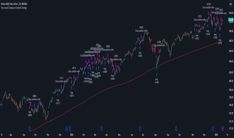
Turn around Tuesday on Steroids Strategy█ STRATEGY DESCRIPTION
The "Turn around Tuesday on Steroids Strategy" is a mean-reversion strategy designed to identify potential price reversals at the start of the trading week. It enters a long position when specific conditions are met and exits when the price shows strength by exceeding the previous bar's high. This strategy is optimized for ETFs, stocks, and other instruments on the daily timeframe.
█ WHAT IS THE STARTING DAY?
The Starting Day determines the first day of the trading week for the strategy. It can be set to either Sunday or Monday, depending on the instrument being traded. For ETFs and stocks, Monday is recommended. For other instruments, Sunday is recommended.
█ SIGNAL GENERATION
1. LONG ENTRY
A Buy Signal is triggered when:
The current day is the first day of the trading week (either Sunday or Monday, depending on the Starting Day setting).
The close price is lower than the previous day's close (`close < close `).
The previous day's close is also lower than the close two days ago (`close < close `).
The signal occurs within the specified time window (between `Start Time` and `End Time`).
If the MA Filter is enabled, the close price must also be above the 200-period Simple Moving Average (SMA).
2. EXIT CONDITION
A Sell Signal is generated when the current closing price exceeds the high of the previous bar (`close > high `). This indicates that the price has shown strength, potentially confirming the reversal and prompting the strategy to exit the position.
█ ADDITIONAL SETTINGS
Starting Day: Determines the first day of the trading week. Options are Sunday or Monday. Default is Sunday.
Use MA Filter: Enables or disables the 200-period SMA filter for long entries. Default is disabled.
Start Time and End Time: The time window during which the strategy is allowed to execute trades.
█ PERFORMANCE OVERVIEW
This strategy is designed for markets with frequent weekly reversals.
It performs best in volatile conditions where price movements are significant at the start of the trading week.
Backtesting results should be analysed to optimize the Starting Day and MA Filter settings for specific instruments.
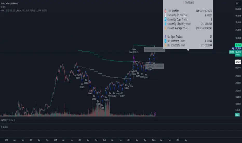
DCA Simulation for CryptoCommunity v1.1Overview
This script provides a detailed simulation of a Dollar-Cost Averaging (DCA) strategy tailored for crypto traders. It allows users to visualize how their DCA strategy would perform historically under specific parameters. The script is designed to help traders understand the mechanics of DCA and how it influences average price movement, budget utilization, and trade outcomes.
Key Features:
Combines Interval and Safety Order DCA:
Interval DCA: Regular purchases based on predefined time intervals.
Safety Order DCA: Additional buys triggered by percentage price drops.
Interactive Visualization:
Displays buy levels, average price, and profit-taking points on the chart.
Allows traders to assess how their strategy adapts to price movements.
Comprehensive Dashboard:
Tracks money spent, contracts acquired, and budget utilization.
Shows maximum amounts used if profit-taking is active.
Dynamic Safety Orders:
Resets safety orders when a new higher high is established.
Customizable Parameters:
Adjustable buy frequency, safety order settings, and profit-taking levels.
Suitable for traders with varying budgets and risk tolerances.
Default Strategy Settings:
Account Size: Default account size is set to $10,000 to represent a realistic budget for the average trader.
Commission & Slippage: Includes realistic trading fees and slippage assumptions to ensure accurate backtesting results.
Risk Management: Defaults to risking no more than 5% of the account balance per trade.
Sample Size: Optimized to generate a minimum of 100 trades for meaningful statistical analysis. Users can adjust parameters to fit longer timeframes or different datasets.
Usage Instructions:
Configure Your Strategy: Set the base order, safety order size, and buy frequency based on your preferred DCA approach.
Analyze Historical Performance: Use the chart and dashboard to understand how the strategy performs under different market conditions.
Optimize Parameters: Adjust settings to align with your risk tolerance and trading objectives.
Important Notes:
This script is for educational and simulation purposes. It is not intended to provide financial advice or guarantee profitability.
If the strategy's default settings do not meet your needs, feel free to adjust them while keeping risk management in mind.
TradingView limits the number of open trades to 999, so reduce the buy frequency if necessary to fit longer timeframes.
One Shot One Kill ICT [TradingFinder] Liquidity MMXM + CISD OTE🔵 Introduction
The One Shot One Kill trading setup is one of the most advanced methods in the field of Smart Money Concept (SMC) and ICT. Designed with a focus on concepts such as Liquidity Hunt, Discount Market, and Premium Market, this strategy emphasizes precise Price Action analysis and market structure shifts. It enables traders to identify key entry and exit points using a structured Trading Model.
The core process of this setup begins with a Liquidity Hunt. Initially, the price targets areas like the Previous Day High and Previous Day Low to absorb liquidity. Once the Change in State of Delivery(CISD)is broken, the market structure shifts, signaling readiness for trade entry. At this stage, Fibonacci retracement levels are drawn, and the trader enters a position as the price retraces to the 0.618 Fibonacci level.
Part of the Smart Money approach, this setup combines liquidity analysis with technical tools, creating an opportunity for traders to enter high-accuracy trades. By following this setup, traders can identify critical market moves and capitalize on reversal points effectively.
Bullish :
Bearish :
🔵 How to Use
The One Shot One Kill setup is a structured and advanced trading strategy based on Liquidity Hunt, Fibonacci retracement, and market structure shifts (CISD). With a focus on precise Price Action analysis, this setup helps traders identify key market movements and plan optimal trade entries and exits. It operates in two scenarios: Bullish and Bearish, each with distinct steps.
🟣 Bullish One Shot One Kill
In the Bullish scenario, the process starts with the price moving toward the Previous Day Low, where liquidity is absorbed. At this stage, retail sellers are trapped as they enter short trades at lower levels. Following this, the market reverses upward and breaks the CISD, signaling a shift in market structure toward bullishness.
Once this shift is identified, traders draw Fibonacci levels from the lowest point to the highest point of the move. When the price retraces to the 0.618 Fibonacci level, conditions for a buy position are met. The target for this trade is typically the Previous Day High or other significant liquidity zones where major buyers are positioned, offering a high probability of price reversal.
🟣 Bearish One Shot One Kill
In the Bearish scenario, the price initially moves toward the Previous Day High to absorb liquidity. Retail buyers are trapped as they enter long trades near the highs. After the liquidity hunt, the market reverses downward, breaking the CISD, which signals a bearish shift in market structure. Following this confirmation, Fibonacci levels are drawn from the highest point to the lowest point of the move.
When the price retraces to the 0.618 Fibonacci level, a sell position is initiated. The target for this trade is usually the Previous Day Low or other key liquidity zones where major sellers are active.
This setup provides a precise and logical framework for traders to identify market movements and enter trades at critical reversal points.
🔵 Settings
🟣 CISD Logical settings
Bar Back Check : Determining the return of candles to identify the CISD level.
CISD Level Validity : CISD level validity period based on the number of candles.
🟣 LIQUIDITY Logical settings
Swing period : You can set the swing detection period.
Max Swing Back Method : It is in two modes "All" and "Custom". If it is in "All" mode, it will check all swings, and if it is in "Custom" mode, it will check the swings to the extent you determine.
Max Swing Back : You can set the number of swings that will go back for checking.
🟣 CISD Display settings
Displaying or not displaying swings and setting the color of labels and lines.
🟣 LIQUIDITY Display settings
Displaying or not displaying swings and setting the color of labels and lines.
🔵 Conclusion
The One Shot One Kill setup is one of the most effective and well-structured trading strategies for identifying and capitalizing on key market movements. By incorporating concepts such as Liquidity Hunt, CISD, and Fibonacci retracement, this setup allows traders to enter trades with high precision at optimal points.
The strategy emphasizes detailed Price Action analysis and the identification of Smart Money behavior, helping traders to execute successful trades against the general market trend.
With a focus on identifying liquidity in the Previous Day High and Low and aligning it with Fibonacci retracement levels, this setup provides a robust framework for entering both bullish and bearish trades.
The combination of liquidity analysis and Fibonacci retracement at the 0.618 level enables traders to minimize risk and exploit major market moves effectively.
Ultimately, success with the One Shot One Kill setup requires practice, patience, and strict adherence to its rules. By mastering its concepts and focusing on high-probability setups, traders can enhance their decision-making skills and build a sustainable and professional trading approach.
